The preceding post is an introduction to order statistics. This post gives examples demonstrating the calculation discussed in the preceding post.
We first work a basic example with a small sample size that walks through all the calculations discussed in the preceding post. More examples are to follow the basic example.
Example 1 – A Basic Example
Suppose that the population distribution is the uniform distribution on the interval 
-
……

……

, respectively. Draw a random sample 


-
……
The support of this joint density is the 3-dimensional region 
The goal here is to derive the density functions of these order statistics and then calculate basic distributional quantities of these order statistics. This is a long example that is presented in five parts – Example 1a through Example 1e.
Example 1a
This example focuses on the minimum statistic.
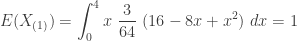
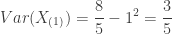
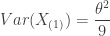
- Compute the mean and variance of the first order statistic
- Compute the conditional probability
.
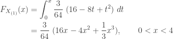
The key step is to derive the density function and the CDF for
-
……
![\displaystyle f_{X_{(1)}}(x)=\frac{3!}{1! \ 2!} \ \frac{1}{4} \ \biggl[1-\frac{x}{4} \biggr]^2=\frac{3}{64} \ (16-8x+x^2) \ \ \ \ \ \ 0<x<4](https://s0.wp.com/latex.php?latex=%5Cdisplaystyle+f_%7BX_%7B%281%29%7D%7D%28x%29%3D%5Cfrac%7B3%21%7D%7B1%21+%5C+2%21%7D+%5C+%5Cfrac%7B1%7D%7B4%7D+%5C+%5Cbiggl%5B1-%5Cfrac%7Bx%7D%7B4%7D+%5Cbiggr%5D%5E2%3D%5Cfrac%7B3%7D%7B64%7D+%5C+%2816-8x%2Bx%5E2%29+%5C+%5C+%5C+%5C+%5C+%5C+0%3Cx%3C4&bg=ffffff&fg=333333&s=0&c=20201002)
The following integrals give the mean and variance of
……
……

……
The following gives the CDF of
-
……
The following gives the conditional probability.
……

Example 1b
This example focuses on the sample median.
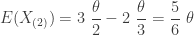
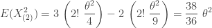
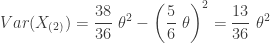
- Compute the mean and variance of the second order statistic
- Compute the conditional probability
.
As in Example 1a, the key step is to find the density function and the CDF.
-
……
![\displaystyle f_{X_{(2)}}(x)=\frac{3!}{1!} \ \frac{x}{4} \ \frac{1}{4} \biggl[1-\frac{x}{4} \biggr]=\frac{6}{64} \ (4x - x^2) \ \ \ \ \ \ 0<x<4](https://s0.wp.com/latex.php?latex=%5Cdisplaystyle+f_%7BX_%7B%282%29%7D%7D%28x%29%3D%5Cfrac%7B3%21%7D%7B1%21%7D+%5C+%5Cfrac%7Bx%7D%7B4%7D+%5C+%5Cfrac%7B1%7D%7B4%7D+%5Cbiggl%5B1-%5Cfrac%7Bx%7D%7B4%7D+%5Cbiggr%5D%3D%5Cfrac%7B6%7D%7B64%7D+%5C+%284x+-+x%5E2%29+%5C+%5C+%5C+%5C+%5C+%5C+0%3Cx%3C4&bg=ffffff&fg=333333&s=0&c=20201002)
……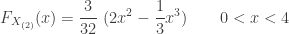
As in Example 1a, evaluating the appropriate integrals and evaluating the CDF appropriately give the desired answers.
-
……

……

……
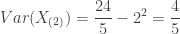
……

Example 1c
This example focuses on the sample maximum.
- Compute the mean and variance of the third order statistic
- Compute the conditional probability
.
The following gives the density function and the CDF of the sample maximum.
-
……
![\displaystyle f_{X_{(3)}}(x)=\frac{3!}{2!} \ \biggl[\frac{x}{4} \biggr]^2 \ \frac{1}{4}=\frac{3}{64} \ x^2 \ \ \ \ \ \ 0<x<4](https://s0.wp.com/latex.php?latex=%5Cdisplaystyle+f_%7BX_%7B%283%29%7D%7D%28x%29%3D%5Cfrac%7B3%21%7D%7B2%21%7D+%5C+%5Cbiggl%5B%5Cfrac%7Bx%7D%7B4%7D+%5Cbiggr%5D%5E2+%5C+%5Cfrac%7B1%7D%7B4%7D%3D%5Cfrac%7B3%7D%7B64%7D+%5C+x%5E2+%5C+%5C+%5C+%5C+%5C+%5C+0%3Cx%3C4&bg=ffffff&fg=333333&s=0&c=20201002)
……
The following gives the desired results after evaluating the integrals and the CDF.
-
……

……

……

……

Example 1d
This example focuses on the joint behavior between the sample minimum and the sample maximum.
- Evaluate the covariance of
- Evaluate the correlation coefficient of
- Compute the conditional probability
.
- Evaluate the conditional mean
.
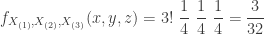
All the calculations in this example are based on the joint density function of the sample minimum and sample maximum.
……
![\displaystyle \begin{aligned} f_{X_{(1)},X_{(3)}}(x,y)&=\frac{3!}{1!} \ \frac{1}{4} \ \biggl[\frac{y}{4}-\frac{x}{4} \biggr] \ \frac{1}{4} \\&=\frac{3}{32} \ (y-x) \ \ \ \ \ \ 0<x<y<4 \end{aligned}](https://s0.wp.com/latex.php?latex=%5Cdisplaystyle+%5Cbegin%7Baligned%7D+f_%7BX_%7B%281%29%7D%2CX_%7B%283%29%7D%7D%28x%2Cy%29%26%3D%5Cfrac%7B3%21%7D%7B1%21%7D+%5C+%5Cfrac%7B1%7D%7B4%7D+%5C+%5Cbiggl%5B%5Cfrac%7By%7D%7B4%7D-%5Cfrac%7Bx%7D%7B4%7D+%5Cbiggr%5D+%5C+%5Cfrac%7B1%7D%7B4%7D+%5C%5C%26%3D%5Cfrac%7B3%7D%7B32%7D+%5C+%28y-x%29+%5C+%5C+%5C+%5C+%5C+%5C+0%3Cx%3Cy%3C4++%5Cend%7Baligned%7D&bg=ffffff&fg=333333&s=0&c=20201002)
The covariance is defined by ![Cov(X_{(1)},X_{(3)})=E[X_{(1)} X_{(3)}]-E[X_{(1)}] E[X_{(3)}]](https://s0.wp.com/latex.php?latex=Cov%28X_%7B%281%29%7D%2CX_%7B%283%29%7D%29%3DE%5BX_%7B%281%29%7D+X_%7B%283%29%7D%5D-E%5BX_%7B%281%29%7D%5D+E%5BX_%7B%283%29%7D%5D&bg=ffffff&fg=333333&s=0&c=20201002)
-
……
![\displaystyle \begin{aligned} E[X_{(1)} X_{(3)}]&=\int_0^4 \int_x^4 x \ y \ f_{X_{(1)},X_{(3)}}(x,y) \ dy \ dx \\&=\int_0^4 \int_x^4 x \ y \ \frac{3}{32} \ (y-x) \ dy \ dx \\&=\int_0^4 \int_x^4 \frac{3}{32} \ (xy^2-x^2 y) \ dy \ dx \\&=\int_0^4 \frac{3}{32} \biggl(\frac{64}{3} x-8x^2+\frac{1}{6} x^4 \biggr) \ dx=\frac{16}{5} \end{aligned}](https://s0.wp.com/latex.php?latex=%5Cdisplaystyle+%5Cbegin%7Baligned%7D+E%5BX_%7B%281%29%7D+X_%7B%283%29%7D%5D%26%3D%5Cint_0%5E4+%5Cint_x%5E4+x+%5C+y+%5C+f_%7BX_%7B%281%29%7D%2CX_%7B%283%29%7D%7D%28x%2Cy%29+%5C+dy+%5C+dx+%5C%5C%26%3D%5Cint_0%5E4+%5Cint_x%5E4+x+%5C+y+%5C+%5Cfrac%7B3%7D%7B32%7D+%5C+%28y-x%29+%5C+dy+%5C+dx+%5C%5C%26%3D%5Cint_0%5E4+%5Cint_x%5E4+%5Cfrac%7B3%7D%7B32%7D+%5C+%28xy%5E2-x%5E2+y%29+%5C+dy+%5C+dx+%5C%5C%26%3D%5Cint_0%5E4+%5Cfrac%7B3%7D%7B32%7D+%5Cbiggl%28%5Cfrac%7B64%7D%7B3%7D+x-8x%5E2%2B%5Cfrac%7B1%7D%7B6%7D+x%5E4+%5Cbiggr%29+%5C+dx%3D%5Cfrac%7B16%7D%7B5%7D+%5Cend%7Baligned%7D&bg=ffffff&fg=333333&s=0&c=20201002)
……
![\displaystyle \begin{aligned} Cov(X_{(1)},X_{(3)})&=E[X_{(1)} X_{(3)}]-E[X_{(1)}] E[X_{(3)}] \\&=\frac{16}{5}-1 \cdot 3=\frac{1}{5} \end{aligned}](https://s0.wp.com/latex.php?latex=%5Cdisplaystyle+%5Cbegin%7Baligned%7D+Cov%28X_%7B%281%29%7D%2CX_%7B%283%29%7D%29%26%3DE%5BX_%7B%281%29%7D+X_%7B%283%29%7D%5D-E%5BX_%7B%281%29%7D%5D+E%5BX_%7B%283%29%7D%5D+%5C%5C%26%3D%5Cfrac%7B16%7D%7B5%7D-1+%5Ccdot+3%3D%5Cfrac%7B1%7D%7B5%7D++%5Cend%7Baligned%7D&bg=ffffff&fg=333333&s=0&c=20201002)
Using the mean and variances from Example 1a and Example 1c, the following shows the calculation for the correlation coefficient.
-
……
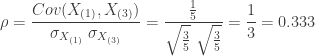
There is a positive correlation between the sample minimum and the sample maximum. This confirms what the natural intuitive idea about the sample minimum and sample maximum. For example, when sample minimum is large, the sample maximum will have to be large as well. Likewise, when sample maximum is small, the sample minimum is also small. However, the correlation is moderate.
To evaluate the conditional probability
-
……
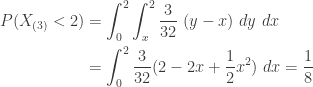
……

……

Based on the CDF in Example 1a, 

……
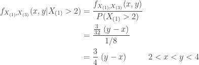
The conditional mean
-
……

From Example 1c, we see that the unconditional mean of 

Example 1e
This example focuses on the sample range 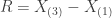
- Evaluate the CDF and the density function of the sample range
.
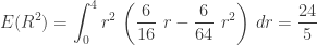
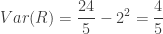
- Determine the mean and variance of the sample range
- Evaluate the conditional mean
.
The CDF of the sample range can be derived by evaluating the following integral (see Fact 5 in the preceding post).
-
……
![\displaystyle F_R(r)=\int_0^4 3 \ [F(x+r)-F(x)]^2 \ f(x) \ dx](https://s0.wp.com/latex.php?latex=%5Cdisplaystyle+F_R%28r%29%3D%5Cint_0%5E4+3+%5C+%5BF%28x%2Br%29-F%28x%29%5D%5E2+%5C+f%28x%29+%5C+dx&bg=ffffff&fg=333333&s=0&c=20201002)
Because the support of the uniform distribution on 


-
……
![\displaystyle \begin{aligned} F_R(r)&=\int_0^4 3 \ [F(x+r)-F(x)]^2 \ f(x) \ dx \\&=\int_0^{4-r} 3 \biggl[\frac{x+r}{4}-\frac{x}{2} \biggr]^2 \ \frac{1}{4} \ dx+\int_{4-r}^4 3 \biggl[1-\frac{x}{4} \biggr]^2 \ \frac{1}{4} \ dx \\&=\int_0^{4-r} \frac{3}{64} r^2 \ dx+\int_{4-r}^4 3 \biggl[1-\frac{x}{4} \biggr]^2 \ \frac{1}{4} \ dx\\&=\frac{3}{64} r^2 (4-r) - \biggl[1-\frac{x}{4} \biggr]^3 \ \biggl \lvert_{4-r}^4 \\&=\frac{3}{16} r^2-\frac{2}{64} r^3 \ \ \ \ \ \ \ 0<r<4 \end{aligned}](https://s0.wp.com/latex.php?latex=%5Cdisplaystyle+%5Cbegin%7Baligned%7D+F_R%28r%29%26%3D%5Cint_0%5E4+3+%5C+%5BF%28x%2Br%29-F%28x%29%5D%5E2+%5C+f%28x%29+%5C+dx+%5C%5C%26%3D%5Cint_0%5E%7B4-r%7D+3+%5Cbiggl%5B%5Cfrac%7Bx%2Br%7D%7B4%7D-%5Cfrac%7Bx%7D%7B2%7D+%5Cbiggr%5D%5E2+%5C+%5Cfrac%7B1%7D%7B4%7D+%5C+dx%2B%5Cint_%7B4-r%7D%5E4+3+%5Cbiggl%5B1-%5Cfrac%7Bx%7D%7B4%7D+%5Cbiggr%5D%5E2+%5C+%5Cfrac%7B1%7D%7B4%7D+%5C+dx+%5C%5C%26%3D%5Cint_0%5E%7B4-r%7D+%5Cfrac%7B3%7D%7B64%7D+r%5E2+%5C+dx%2B%5Cint_%7B4-r%7D%5E4+3++%5Cbiggl%5B1-%5Cfrac%7Bx%7D%7B4%7D+%5Cbiggr%5D%5E2+%5C+%5Cfrac%7B1%7D%7B4%7D+%5C+dx%5C%5C%26%3D%5Cfrac%7B3%7D%7B64%7D+r%5E2+%284-r%29+-+%5Cbiggl%5B1-%5Cfrac%7Bx%7D%7B4%7D+%5Cbiggr%5D%5E3+%5C++%5Cbiggl+%5Clvert_%7B4-r%7D%5E4+%5C%5C%26%3D%5Cfrac%7B3%7D%7B16%7D+r%5E2-%5Cfrac%7B2%7D%7B64%7D+r%5E3+%5C+%5C+%5C+%5C+%5C+%5C+%5C+0%3Cr%3C4+%5Cend%7Baligned%7D&bg=ffffff&fg=333333&s=0&c=20201002)
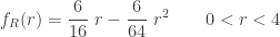
The density function 
-
……
……

……
……
……

Observe that the unconditional mean of the sample range is 2 while the mean is 2.75 given that the sample range is larger than 2.
More Examples
Example 1 is a long example demonstrating all the basic calculations with sampling from a uniform distribution. The next several examples involves sampling from an exponential distribution.
Example 2
Let 


The density function and the CDF of the exponential population are:
-
……

……
The following gives the density functions of the three order statistics.
-
……

……

……
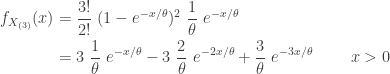
Note that the density 

-
……

……
Note that both 

-
……
……
……
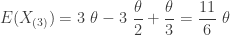
Using the same thought process, the following gives the mean and variance of
-
……
……

……

We make additional comments about these order statistics in the section below called “A Comparison of Estimators”.
Example 3
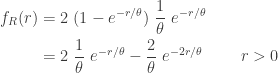
This is a continuation of Example 2. Consider the sample range
The CDF of the sample range can be derived by evaluating the following integral (see Fact 5 in the preceding post).
-
……
![\displaystyle F_R(r)=\int_0^\infty 3 \ [F(x+r)-F(x)]^2 \ f(x) \ dx](https://s0.wp.com/latex.php?latex=%5Cdisplaystyle+F_R%28r%29%3D%5Cint_0%5E%5Cinfty+3+%5C+%5BF%28x%2Br%29-F%28x%29%5D%5E2+%5C+f%28x%29+%5C+dx&bg=ffffff&fg=333333&s=0&c=20201002)
Because the support of the exponential distribution is unbounded above, there is no need to split the integral.
-
……
![\displaystyle \begin{aligned} F_R(r)&=\int_0^\infty 3 \ [e^{-x/\theta}-e^{-(x+r)/\theta}]^2 \ \frac{1}{\theta} \ e^{-x/\theta} \ dx \\&=\int_0^\infty 3 \ e^{-2x/\theta} \ (1-e^{-r/\theta})^2 \ \frac{1}{\theta} e^{-x/\theta} \ dx \\&=\int_0^\infty \frac{3}{\theta} \ e^{-3x/\theta} \ (1-e^{-r/\theta})^2 \ dx \\&=(1-e^{-r/\theta})^2 \ \ \ \ \ \ \ r>0 \end{aligned}](https://s0.wp.com/latex.php?latex=%5Cdisplaystyle+%5Cbegin%7Baligned%7D+F_R%28r%29%26%3D%5Cint_0%5E%5Cinfty+3+%5C+%5Be%5E%7B-x%2F%5Ctheta%7D-e%5E%7B-%28x%2Br%29%2F%5Ctheta%7D%5D%5E2+%5C+%5Cfrac%7B1%7D%7B%5Ctheta%7D+%5C+e%5E%7B-x%2F%5Ctheta%7D+%5C+dx+%5C%5C%26%3D%5Cint_0%5E%5Cinfty+3+%5C+e%5E%7B-2x%2F%5Ctheta%7D+%5C+%281-e%5E%7B-r%2F%5Ctheta%7D%29%5E2+%5C+%5Cfrac%7B1%7D%7B%5Ctheta%7D+e%5E%7B-x%2F%5Ctheta%7D+%5C+dx+%5C%5C%26%3D%5Cint_0%5E%5Cinfty+%5Cfrac%7B3%7D%7B%5Ctheta%7D+%5C+e%5E%7B-3x%2F%5Ctheta%7D+%5C+%281-e%5E%7B-r%2F%5Ctheta%7D%29%5E2+%5C+dx+%5C%5C%26%3D%281-e%5E%7B-r%2F%5Ctheta%7D%29%5E2+%5C+%5C+%5C+%5C+%5C+%5C+%5C+r%3E0++%5Cend%7Baligned%7D&bg=ffffff&fg=333333&s=0&c=20201002)
Differentiating the CDF producing the density function. The following also shows the mean and variance of the sample range.
……
……

……

……

Example 4
This is a continuation of Example 2 and Example 3. Use the sample range 
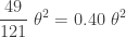
The covariance of
-
……

Computing 
-
……

All the variance terms are easily accessible (and have been calculated). Thus we can solve for the covariance term.
-
……

The following gives the correlation coefficient.
-
……

The correlation between the sample minimum and sample maximum is quite moderate.
Example 5
Examples 2, 3 and 4 are based on a small sample size sampling from the exponential population. We now look at sampling from exponential distribution in general, i.e. the sample size is arbitrary. Let 

As shown in Example 3, the CDF of the sample range is obtained by evaluating the following integral.
-
……
![\displaystyle F_R(r)=\int_0^\infty n \ [F(x+r)-F(x)]^{n-1} \ f(x) \ dx](https://s0.wp.com/latex.php?latex=%5Cdisplaystyle+F_R%28r%29%3D%5Cint_0%5E%5Cinfty+n+%5C+%5BF%28x%2Br%29-F%28x%29%5D%5E%7Bn-1%7D+%5C+f%28x%29+%5C+dx&bg=ffffff&fg=333333&s=0&c=20201002)
This integral is quite similar to the one in Example 3 and is evaluated in the same manner.
-
……
![\displaystyle \begin{aligned} F_R(r)&=\int_0^\infty n \ [e^{-x/\theta}-e^{-(x+r)/\theta}]^{n-1} \ \frac{1}{\theta} \ e^{-x/\theta} \ dx \\&=\int_0^\infty n \ e^{-(n-1)x/\theta} \ (1-e^{-r/\theta})^{n-1} \ \frac{1}{\theta} e^{-x/\theta} \ dx \\&=\int_0^\infty \frac{n}{\theta} \ e^{-nx/\theta} \ (1-e^{-r/\theta})^{n-1} \ dx \\&=(1-e^{-r/\theta})^{n-1} \ \ \ \ \ \ \ r>0 \end{aligned}](https://s0.wp.com/latex.php?latex=%5Cdisplaystyle+%5Cbegin%7Baligned%7D+F_R%28r%29%26%3D%5Cint_0%5E%5Cinfty+n+%5C+%5Be%5E%7B-x%2F%5Ctheta%7D-e%5E%7B-%28x%2Br%29%2F%5Ctheta%7D%5D%5E%7Bn-1%7D+%5C+%5Cfrac%7B1%7D%7B%5Ctheta%7D+%5C+e%5E%7B-x%2F%5Ctheta%7D+%5C+dx+%5C%5C%26%3D%5Cint_0%5E%5Cinfty+n+%5C+e%5E%7B-%28n-1%29x%2F%5Ctheta%7D+%5C+%281-e%5E%7B-r%2F%5Ctheta%7D%29%5E%7Bn-1%7D+%5C+%5Cfrac%7B1%7D%7B%5Ctheta%7D+e%5E%7B-x%2F%5Ctheta%7D+%5C+dx+%5C%5C%26%3D%5Cint_0%5E%5Cinfty+%5Cfrac%7Bn%7D%7B%5Ctheta%7D+%5C+e%5E%7B-nx%2F%5Ctheta%7D+%5C+%281-e%5E%7B-r%2F%5Ctheta%7D%29%5E%7Bn-1%7D+%5C+dx+%5C%5C%26%3D%281-e%5E%7B-r%2F%5Ctheta%7D%29%5E%7Bn-1%7D+%5C+%5C+%5C+%5C+%5C+%5C+%5C+r%3E0++%5Cend%7Baligned%7D&bg=ffffff&fg=333333&s=0&c=20201002)
Thus the CDF of the sample range when sampling from an exponential population is simply the CDF of the exponential population raised to the sample size less one. Interestingly the CDF of the sample maximum when sampling from exponential distribution looks similar, except that the power is the sample size 
-
……

Of course, the distributional form may look the same, the sample range and the sample maximum have different distributions.
A Comparison of Estimators
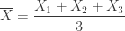
We close out the post by commenting on Example 2. Recall that Example 2 focuses on the means and variances of the three order statistics when sampling from an exponential distribution with the sample size being 3. We now compare these three order statistics with the sample mean, which in this case is the sum of the three sample items divided by 3.
-
……
Of course, the sample mean 
-
……

……

The sample mean as an estimator of
The following table lists out the means and variances of
| Statistic | …… | …… | …… | …… | Mean | …… | …… | …… | …… | Variance |
|---|---|---|---|---|---|---|---|---|---|---|
|
…… | …… | …… | …… | |
…… | …… | …… | …… |  |
| …… | …… | …… | …… | …… | …… | …… | …… | …… | …… | …… |
|
…… | …… | …… | …… |  |
…… | …… | …… | …… |  |
| …… | …… | …… | …… | …… | …… | …… | …… | …… | …… | …… |
|
…… | …… | …… | …… |  |
…… | …… | …… | …… |  |
| …… | …… | …… | …… | …… | …… | …… | …… | …… | …… | …… |
|
…… | …… | …… | …… |  |
…… | …… | …… | …… |  |
The sample minimum
Thus the three order statistics are not so desirable as estimators of the population mean of an exponential population as they are biased estimators of the population mean
| Statistic | …… | …… | …… | …… | Mean | …… | …… | …… | …… | Variance |
|---|---|---|---|---|---|---|---|---|---|---|
|
…… | …… | …… | …… | |
…… | …… | …… | …… |  |
| …… | …… | …… | …… | …… | …… | …… | …… | …… | …… | …… |
 |
…… | …… | …… | …… |  |
…… | …… | …… | …… |  |
| …… | …… | …… | …… | …… | …… | …… | …… | …… | …… | …… |
 |
…… | …… | …… | …… | |
…… | …… | …… | …… |  |
| …… | …… | …… | …… | …… | …… | …… | …… | …… | …… | …… |
 |
…… | …… | …… | …… | |
…… | …… | …… | …… |  |
The above table shows that all 4 statistics (or estimators) have the same expected value. On average they are correct. Now that we have four unbiased estimators of the same parameter
When the competing estimators are all unbiased estimators of the same target parameter, what is another property that can distinguish among the seemingly similar estimators? When the estimators are all unbiased, we would prefer the estimator that has the smallest variance. This is because using an estimator with a smaller variance guarantees that in repeated sampling a higher proportion of the values of the estimator will be close to the target parameter. Thus, the estimator with the smallest variance is the one that will more likely to produce good estimates. In addition to unbiasedness, we would prefer the variance of the distribution of the estimator to have a variance that is as small as possible.
Let’s look at the variance of these four estimators. The last table shows that the sample mean 
Even though the order statistics are not good candidate of the exponential population mean, there are situations where order statistics are good candidates for statistical estimation. The examples of order statistics in this post are also convenient examples for demonstrating the notions of unbiased estimators and the notion that smaller variance is better in comparing two estimators that are otherwise similar.
Practice problems on order statistics are found in this companion blog.
Dan Ma math
Daniel Ma mathematics
Dan Ma stats
Daniel Ma statistics
Dan Ma statistical
Daniel Ma statistical


Pingback: Estimating percentiles using order statistics | Mathematical Statistics